Traffic Accident Severity Prediction

In one minute

The essentials, for someone who won't read the full report.

Problem

Predict the maximum injury severity of a traffic crash — no injury, minor, severe, or fatal — from crash-level records. Fatal crashes make up only ~2.4% of cases.

Dataset

101,904 police-reported U.S. crashes from the Crash Report Sampling System (CRSS, 2016–2023), flattened from 28 relational tables into 163 features.

Models

A class-weighted Linear SVM and an ordinal XGBoost pipeline that decomposes the 4-class problem into three cumulative binary classifiers.

Explainability

SHAP for global feature attribution, LIME for local instance-level explanations, and DiCE for counterfactuals — plus an explanation-driven feature-reduction test.

Takeaway

Both models reach ≈0.59 accuracy / 0.53–0.54 macro-F1. Oversampling lifts fatal-class F1 from 0.26 to 0.59 — but feature reduction doesn't generalize.

Why recall matters more than precision here. Correctly identifying fatal injuries is of paramount importance: predicting a non-fatal case as fatal has far less severe consequences than missing a truly fatal one. That asymmetry shaped both the evaluation (macro-F1, per-class F1) and the oversampling strategy.

Dataset & task

Official U.S. police-reported crash records, released as the Crash Report Sampling System (CRSS). The raw data are 28 relational tables — ACCIDENT, VEHICLE, PERSON, and more — linked by a unique crash identifier.

101,904 crashes in the full dataset

163 crash-level features

28 relational source tables

40.9% of records contain an unknown indicator

From tables to vectors. Each crash becomes one feature vector: entity-level attributes (vehicles, drivers, occupants) are aggregated to the crash level as counts, proportions, and summary statistics, with indexed slots for repeated roles (TRAV_SP_1, TRAV_SP_2, …). The target is MAX_SEV — the maximum injury severity in the crash — remapped to an ordered four-class label: 0 no injury, 1 minor, 2 severe, 3 fatal (with “possible injury” merged into minor).

Missingness is encoded, not hidden. Structured unknowns become explicit _UNKNOWN (attribute missing) and _NOT_APPLICABLE (conceptually irrelevant) indicator features — and they turn out to carry predictive signal of their own (see Explainability). Two data representations are kept apart: a leakage-safe predictive feature set, and an imputed, explanation-only view used for LIME and DiCE.

Class imbalance and SMOTE. A SMOTE-oversampled variant is created on the training split only, raising fatal prevalence from 2.38% to 5.38% — about half the prevalence of the severe class, rather than full balancing. Both variants are trained and compared side by side.

Class distribution — held-out test split

0 — no injury 48.87%

1 — minor 37.69%

2 — severe 11.08%

3 — fatal 2.37%

Splits — train 71,332 · validation 15,286 · test 15,286 (final report, Table 1)

Why SVM and XGBoost

The final report picks up the story after the finalists were chosen. This is how they were chosen — five model families screened head to head.

Preliminary analysis — 20k subset (batch_1), progress stage

Selected for the final study Screened out

Logistic regression 0.378

Linear SVM 0.384

Linear SVM + SMOTE 0.443

Nyström SVM (kernel approx.) 0.419

Random Forest (best config) 0.396

XGBoost (cumulative + SMOTE) 0.450

Macro-F1, best configuration per family — progress report ablation tables

What the screening showed. Strong, interpretable baselines held their own against heavier models: kernel-approximated SVMs and tuned Random Forests bought little over a plain linear SVM, while a cumulative (ordinal) XGBoost variant led the field. SMOTE helped every minority class everywhere it was applied. The team carried the two most complementary survivors — a linear model and an ordinal gradient-boosted ensemble — into the full-dataset study.

Random Forest SHAP summary for the fatal class — **Fig. S1** — Random Forest SHAP, fatal class (screening stage; 20k subset)

Methodology

Fixed train/validation/test splits; both oversampling settings; explainability aggregated over a fixed evaluation subset; final models re-trained with reduced features and re-evaluated on the held-out test set.

28 CRSS tablescrash · vehicle · person

→

Crash-level vector163 features · indexed slots + aggregates

→

Train / val / test71k / 15k / 15k

→

± SMOTEtrain split only

→

Linear SVM ∥ Ordinal XGBoost

→

SHAP · LIME · DiCE

Linear SVM

Class-weighted (class_weight=balanced) to counter the 2.4% fatal class.
C tuned on validation over a logarithmic grid; numeric features scaled, categoricals encoded.
Best macro-F1 among the linear baselines in the screening stage.
Gets class-conditional explanations — separate SHAP/LIME views per severity class.

Ordinal XGBoost

Cumulative decomposition into three binary subproblems: P(y≥1), P(y≥2), P(y≥3).
Separate classifier per threshold, early stopping on validation, scale_pos_weight per binary distribution.
Class probabilities by subtraction — P(y=0)=1−p₁, P(y=1)=p₁−p₂, P(y=2)=p₂−p₃, P(y=3)=p₃ — argmax decision.
Respects the ordering of severity classes that plain multiclass ignores.

Explainability

Three complementary lenses: SHAP explains the model globally, LIME explains single predictions locally, and DiCE asks what would have to change for a prediction to move away from fatal.

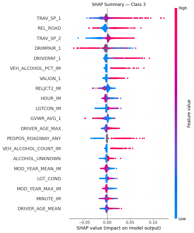
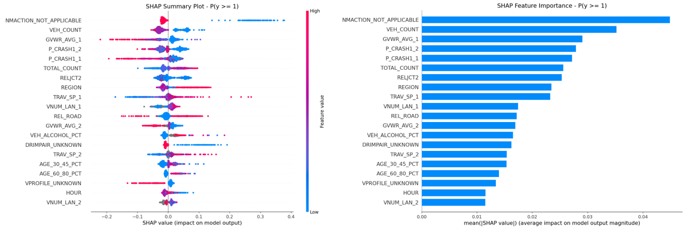
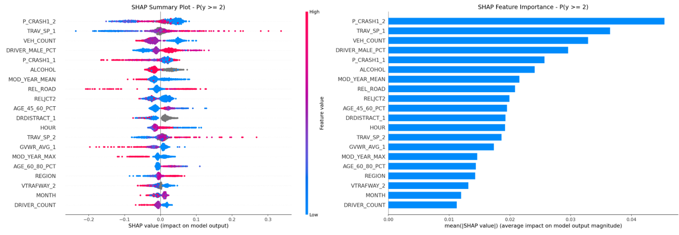
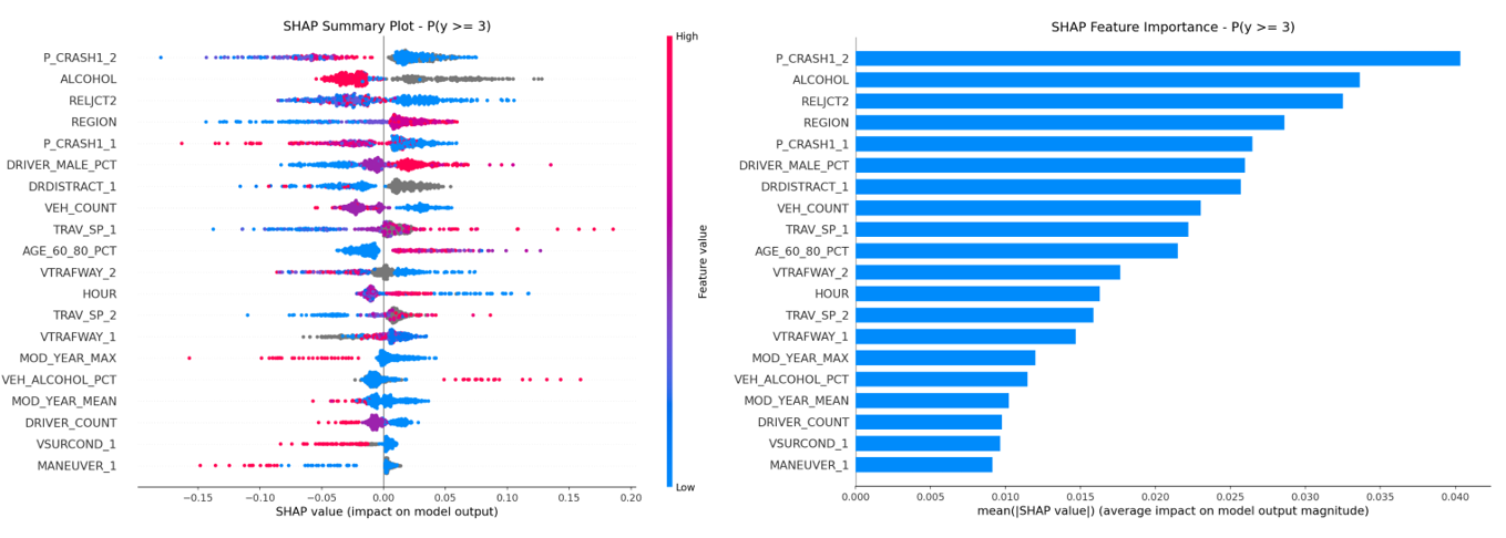
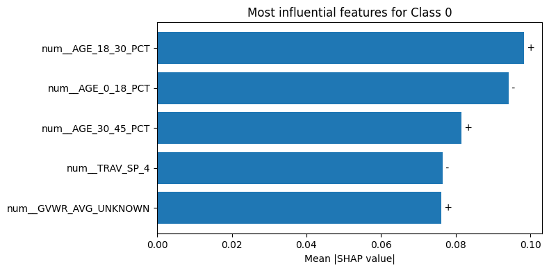
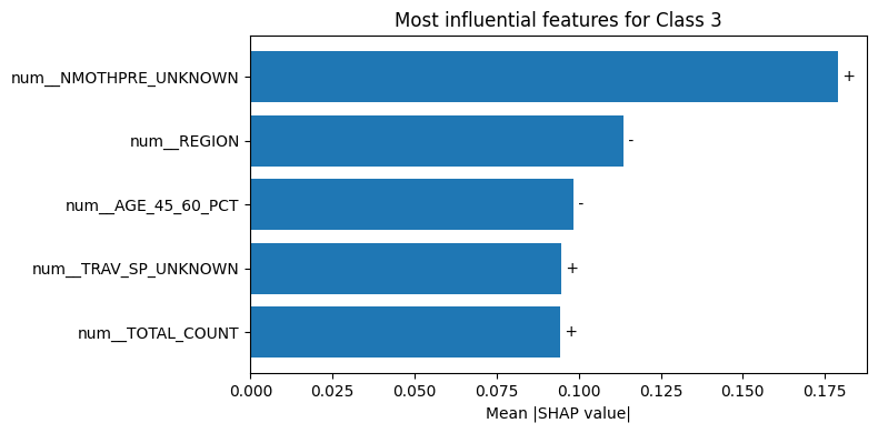
Global feature attribution on the predictive feature space (mean absolute SHAP). For XGBoost, importances are computed per ordinal threshold; the most influential features include NMACTION_NA, VEH_COUNT, GVWR_AVG_1, ALCOHOL, DRDISTRACT_1, and the travel-speed slots TRAV_SP_*. The SVM is explained class-conditionally — the fatal class is pushed upward by TOTAL_COUNT and NMOTHPRE_UNKNOWN, and downward by REGION and the 45–60 age-share.

XGBoost SHAP summary for P(y≥1) — **Fig. 2a** — XGBoost Variant A, SHAP for P(y≥1): any injury

XGBoost SHAP summary for P(y≥2) — **Fig. 2b** — SHAP for P(y≥2): severe or fatal

XGBoost SHAP summary for P(y≥3) — **Fig. 2c** — SHAP for P(y≥3): the fatal threshold

SVM SHAP top features for class 0 — **Fig. 5a** — SVM SHAP, class 0 (no injury)

SVM SHAP top features for class 3 — **Fig. 5b** — SVM SHAP, class 3 (fatal)

Preliminary analysis — 20k subset (batch_1), progress stage

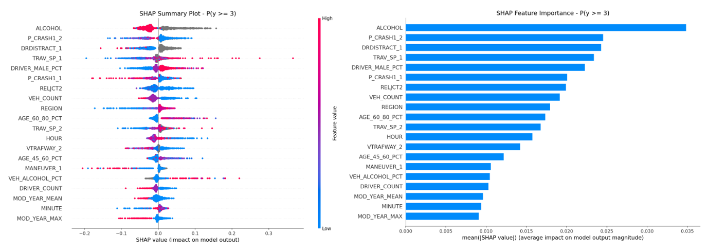
Missingness itself is a signal. An ablation from the progress stage removed every *_UNKNOWN indicator from the XGBoost model. Use the toggle: with the indicators present, the fatal-threshold model leans heavily on reporting artifacts (NMHELMET_UNKNOWN, NMACTION_UNKNOWN); without them, substantive factors like ALCOHOL dominate — at a small cost in macro-F1 (0.45 → 0.44 on the subset).

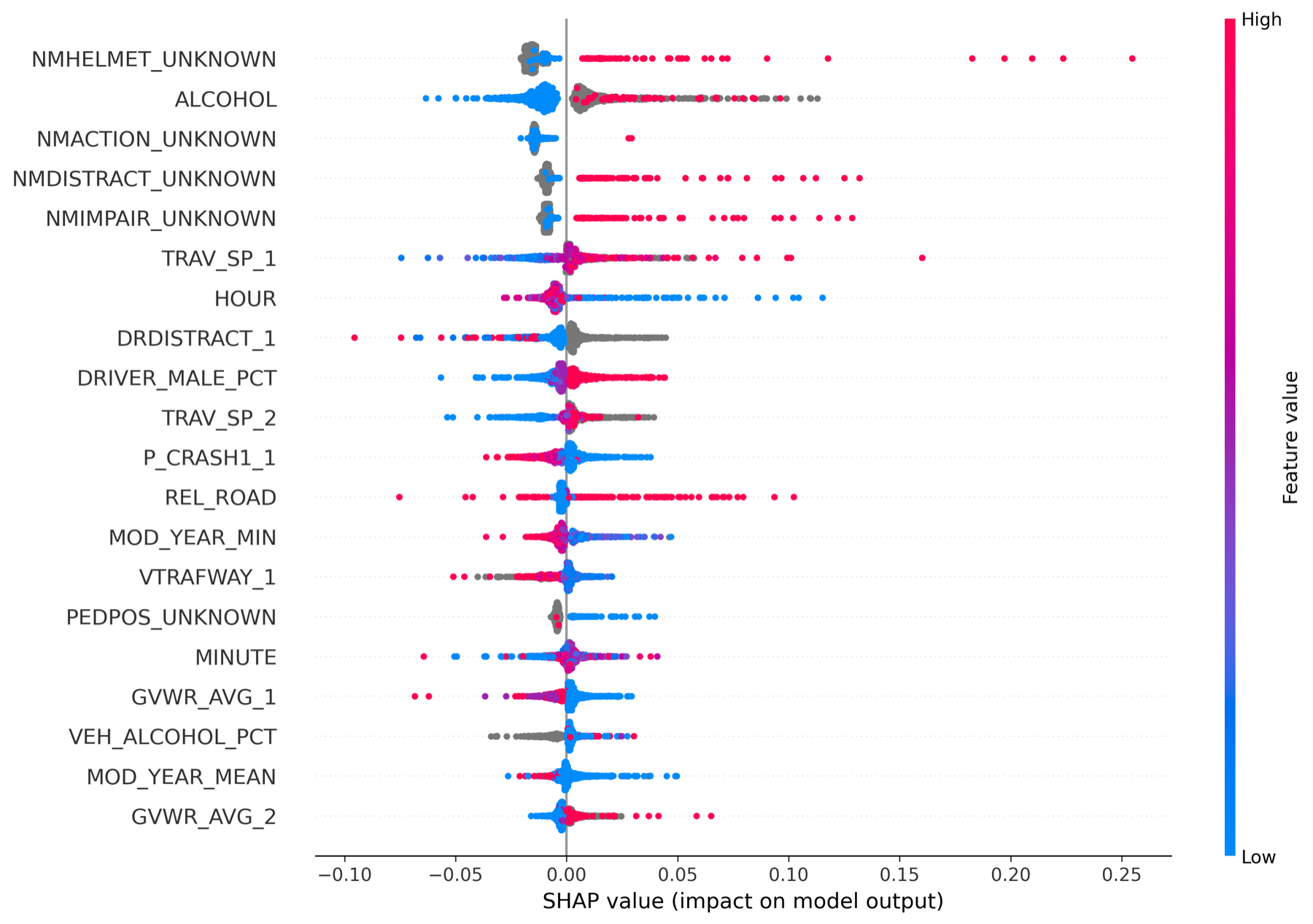
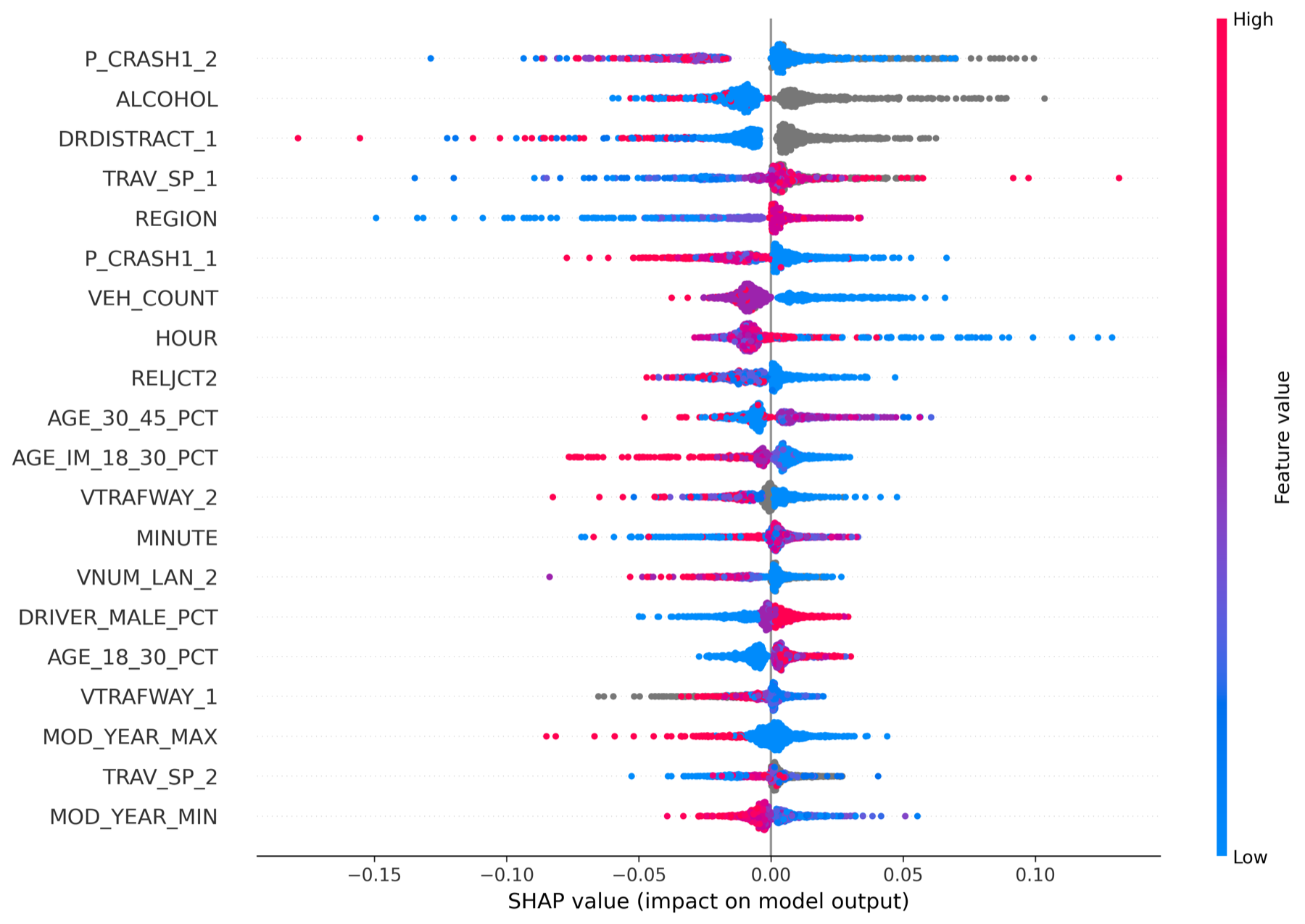
SHAP summary for P(y≥3) including unknown indicators

SHAP summary for P(y≥3) after removing unknown indicators

XGBoost SHAP for the fatal threshold P(y≥3), before / after removing *_UNKNOWN features — progress report, Model 8 vs. Model 8′ (20k subset).

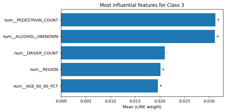
Local, instance-level explanations on the imputed explanation-only representation. XGBoost LIME weights were aggregated over a fixed set of 89 evaluation instances — VTRAFWAY_4, PEDESTRIAN_COUNT, and P_CRASH1_4 recur most strongly — while the SVM was explained class-conditionally for qualitative case studies.

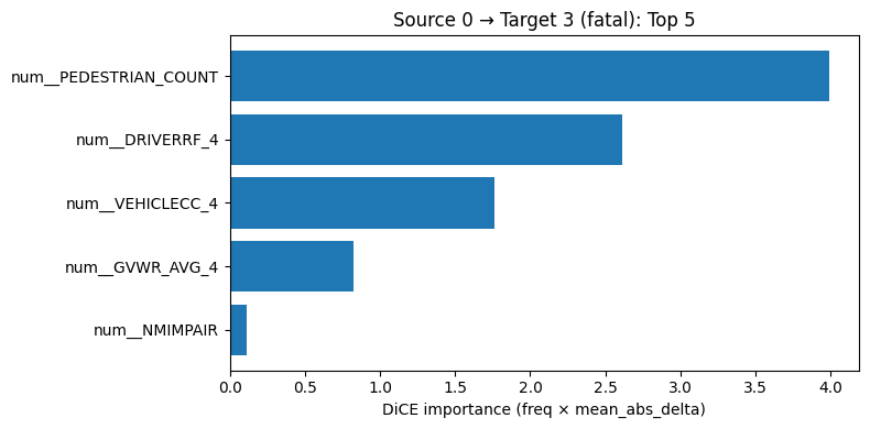
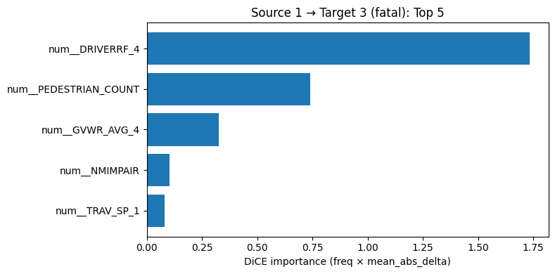
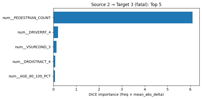
SVM LIME explanation for class 3 — **Fig. 7** — SVM LIME, class 3 (fatal)

DiCE generates counterfactuals targeting the fatal class: for 20 truly fatal test crashes, three counterfactuals each, asking what minimal changes move the prediction away from fatal? For XGBoost, P_CRASH1_2, MANEUVER_1, and DRIVER_DRUGS_PCT are changed most often; for the SVM, PEDESTRIAN_COUNT, DRIVERRF_4, and VEHICLECC_4 dominate. The report is explicit about the caveat: these are decision-boundary sensitivities, not causal mechanisms.

SVM DiCE most important features, source class 0 — **Fig. 8a** — DiCE, source class 0 → fatal

SVM DiCE most important features, source class 1 — **Fig. 8b** — DiCE, source class 1 → fatal

SVM DiCE most important features, source class 2 — **Fig. 8c** — DiCE, source class 2 → fatal

Results & findings

All numbers below are the final, full-dataset results exactly as reported — validation unless marked test.

≈0.59 accuracy, both models (oversampled eval)

0.53–0.54 macro-F1, both models (oversampled eval)

0.26 → 0.59 fatal-class F1, XGBoost without → with SMOTE

163 → 154 features after explanation-driven reduction (XGB)

Validation confusion matrices for XGBoost Variant A, Variant B, and SVM — **Fig. 1** — Validation confusion matrices: XGBoost Var A · Var B · SVM

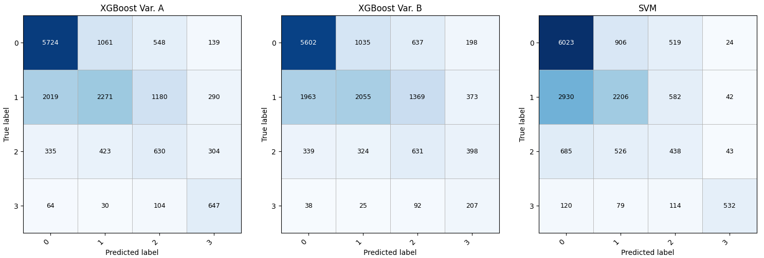
Oversampling, class by class — XGBoost per-class F1

Variant A — oversampled Variant B — non-oversampled

C0 · no injury — A 0.734

C0 · no injury — B 0.734

C1 · minor — A 0.460

C1 · minor — B 0.447

C2 · severe — A 0.315

C2 · severe — B 0.289

C3 · fatal — A 0.595

C3 · fatal — B 0.264

Validation, XGBoost Variant A vs Variant B — final report, Table 8

Model	Macro-F1	Weighted-F1
XGBoost Var A (oversampled)	0.5235	0.5849
XGBoost Var B (non-oversampled)	0.4321	0.5616
Linear SVM	0.5356	0.5678

Final report, Table 2

Metric	Full (163 feat.)	Reduced (154 feat.)
F1 — C0 no injury	0.726334	0.725452
F1 — C1 minor	0.422237	0.422542
F1 — C2 severe	0.274283	0.274321
F1 — C3 fatal	0.514220	0.507269
Macro F1	0.484269	0.482396
Weighted F1	0.555334	0.554659

Final report, Table 9 — reduction removes features consistently negligible across SHAP/LIME/DiCE

Metric	XGBoost Full	XGBoost Reduced	SVM Full
F1 — C0 no injury	0.726334	0.725452	0.700000
F1 — C1 minor	0.422237	0.422542	0.450000
F1 — C2 severe	0.274283	0.274321	0.220000
F1 — C3 fatal	0.514220	0.507269	0.400000
Macro F1	0.484269	0.482396	0.445644
Weighted F1	0.555334	0.554659	0.540000
# Features	163	154	163

Final report, Table 11 — evaluated on the test set

Findings & limitations

Oversampling's benefit is concentrated on the fatal class — fatal F1 rises 0.264 → 0.595 while the majority classes are essentially unchanged.
Both models struggle most with adjacent mid classes — minor vs severe confusion is the main residual error, as the confusion matrices show.
Explanation-driven feature elimination does not improve generalization (XGBoost test macro-F1 0.4843 → 0.4824; SVM validation 0.5356 → 0.5321 even after cutting 163 → 55 features) — the signal is distributed across many features, so SHAP/LIME/DiCE serve best as interpretation tools, not selection mechanisms.
Counterfactuals are not causes. DiCE reflects model sensitivity at the decision boundary, and the missingness markers (*_UNKNOWN) are themselves predictive — both demand careful interpretation.
Future work: more explicitly ordinal and cost-sensitive training to reduce mid-class confusion, better calibration for minority-class decisions, and richer contextual features.

Figure gallery

Every figure used on this page, with its original caption context. Click any figure to inspect it at full size.

Validation confusion matrices — **Fig. 1** — Confusion matrices, validation

Random Forest SHAP summary, fatal class — **Fig. S1** — RF SHAP, fatal (preliminary)

XGBoost SHAP P(y≥1) — **Fig. 2a** — XGB SHAP, P(y≥1)

XGBoost SHAP P(y≥2) — **Fig. 2b** — XGB SHAP, P(y≥2)

XGBoost SHAP P(y≥3) — **Fig. 2c** — XGB SHAP, P(y≥3)

XGBoost reduced-model SHAP P(y≥3) — **Fig. 4** — XGB reduced, SHAP P(y≥3)

SVM SHAP class 0 — **Fig. 5a** — SVM SHAP, class 0

SVM SHAP class 3 — **Fig. 5b** — SVM SHAP, class 3

SVM LIME class 3 — **Fig. 7** — SVM LIME, class 3

SVM DiCE source class 0 — **Fig. 8a** — DiCE, class 0 → fatal

SVM DiCE source class 1 — **Fig. 8b** — DiCE, class 1 → fatal

SVM DiCE source class 2 — **Fig. 8c** — DiCE, class 2 → fatal

Materials

The full report as submitted for CS512 (Machine Learning), Sabancı University, January 2026 — Sima Adleyba, Başak Çarhacıoğlu, Ahmet İhsan Gül.

Model Selection and Explainability in Traffic Accident Severity Prediction

Final report · 11 pages · PDF · January 2026

Download ↓ View in browser ↗

Figures and numbers on this page are taken from the final report; blocks marked “Preliminary analysis” come from the project's earlier progress stage, which ran on a representative 20k subset before scaling to the full dataset. There is no public code repository for this project.